Introduction to Computing for Engineers and Computer Scientists

HW2, Algorithms, Some Libraries

Questions, Comments

Questions from Class

Piazza Questions

Type Checking

Question

Checking Types

• This question will become tricky when we start using classes. (Punch and Enbody, Chpt. 11)

• Any object (variable or literal) we have seen so far is of a simple type, e.g. float, int, ...

• Classes allow programmer defined types, and an object can simultaneously have several types.

Short Answer

• For now, you can use the built in function isinstance().

isinstance(1,int)

True

isinstance(3.2,float)

True

isinstance(3.2,int)

False

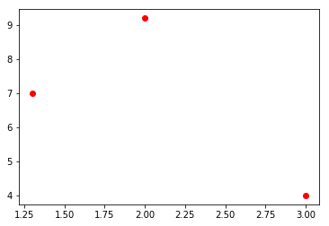
An Example

import matplotlib.pyplot as plt

def add_to_plot(x,y):
    result = False
    if (isinstance(x,int) or isinstance(x,float)) and \
        (isinstance(y,int) or isinstance(y,float)):
        plt.plot(x,y,"ro")
        result = True
        
    return result

x = 3
y = 4

if add_to_plot(x,y):
    print("Plotted ",x,",",y)
else:
    print("Plotting ",x,",",y,"failed!")
    
x = 2
y = 9.2

if add_to_plot(x,y):
    print("Plotted ",x,",",y)
else:
    print("Plotting ",x,",",y,"failed!")
    
    
x = 1.3
y = 7

if add_to_plot(x,y):
    print("Plotted ",x,",",y)
else:
    print("Plotting ",x,",",y,"failed!")

x = 'c'
y = 7

if add_to_plot(x,y):
    print("Plotted ",x,",",y)
else:
    print("Plotting ",x,",",y,"failed!")
    
    
plt.show()

Plotted  3 , 4
Plotted  2 , 9.2
Plotted  1.3 , 7
Plotting  c , 7 failed!

Longer Answer -- Duck Typing

• Duck Typing? I am not kidding.

• Duck Typing: "Duck typing is concerned with establishing the suitability of an object for some purpose, using the principle, "If it walks like a duck and it quacks like a duck, then it must be a duck." With normal typing, suitability is assumed to be determined by an object's type only. In duck typing, an object's suitability is determined by the presence of certain methods and properties (with appropriate meaning), rather than the actual type of the object."

• What does this mean? Try to use it like a duck, and if explodes, it was not a duck. I am not kidding.

import matplotlib.pyplot as plt

try:
    x,y = 1.1, 3
    plt.plot(x,y,"ro")
    x,y = 3.2, 5
    plt.plot(x,y,"ro")
    x,y = 'a','yellow'
    plt.plot(x,y,"ro")
    plt.show()
except ValueError as ve:
    print("Got value error = ",ve)
finally:
    print("Either ",x,"or",y,"was not a duck.")
    

Got value error =  could not convert string to float: 'a'
Either  a or yellow was not a duck.

Python Features

Python Features

• Every (almost) every feature in Python exists in other languages.

• We covered this course's choice of Python in the 1st lecture.

• The example of a,b = b,a is a specific case off a,b = <expresion>
  • This syntax and capability is unusual.
  • Some other languages support it, e.g. Lua

• Languages implement statements by parsing and code generation.
  • The basic syntax is LHS = <expression>
  • Simplistically, the steps in the evaluation of x = 1 + 2 are
    1. Evaluate the expression 1 + 2 and create a new object with the value.
    2. Change x to reference the new object.
    3. Delete/release the previous object x referenced, if not other variable references it.
  • The generated code evaluates the <expression> and produces an object, and then changes the variable to reference the object.

• This is what Python does but extends to LHS1, LHS2, LHS2 = <expression1>, <expression2>, <expression3>

• The generated code evaluates all of the expressions and creates the result objects, _and then has the LHS reference the result expressions.

• Just like a + b, a is an expression.

a = 3

# a is an expression. Evaluate a.
a

3

• Overly simplistically, for a,b = b,a Python parses and produces the following code
  1. Evaluate the expression b and produce a new object o1 with the value.
  2. Evaluate the expression a and produce a new object o2 with the value.
  3. Change a to reference o1
  4. Change b to reference o2

• Is this syntax and feature useful? Some people argue "yes" and some people argue "no."

• What do I think? Well,
  • I am old $\Rightarrow$ I think all new things are a bad idea.
  • I am from rural New England $\Rightarrow$ I am cranky and dislike everything.
  • My ancestry is Scottish $\Rightarrow$ I am cranky and dislike everything.
  • I am not entirely sure computers are not a bad idea.
  • Use the feature if you want. Avoid it if you want.

• The feature most commonly appears in function returns.

# Multiple return example
def three_powers(x):
    r1 = x**2
    r2 = x**3
    r3 = x**3
    
    return r1, r2, r3

# More "traditional" multiple return approach
def another_three_powers(x):
    r1 = x**2
    r2 = x**3
    r3 = x**3
    
    return [r1, r2, r3]

print("Multiple returns = ", three_powers(2))
print("Cranky, old guy multiple returns = ", another_three_powers(2))

Multiple returns =  (4, 8, 8)
Cranky, old guy multiple returns =  [4, 8, 8]

• Hmm. I did not expect the parentheses.

a = 1
b = 2

a,b

(1, 2)

x = 3
y = 4
(x , y) = (y, x)
y,x

(3, 4)

• If you decide not to use the multiple assignment syntax,
  • You need to be aware of it because
  • You may use code or a library that someone else wrote, and they like multiple returns.

Deconstructing HW2

Geometric Brownian Motion

Explanation

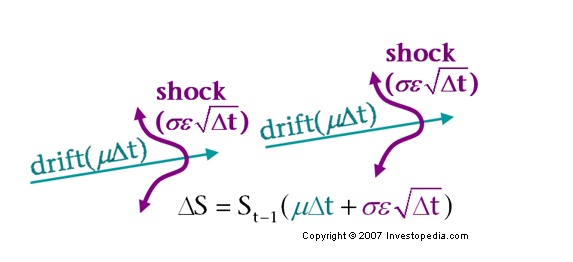
• Investopedia (Yes, that is really a thing) has a good explanation of Monet Carlo simulation of stock price evolution.

• The formula \begin{equation} S_t = S_{t-1} * (1 + \mu\delta t + \sigma\phi \sqrt{\delta t}) \end{equation}

• Is the same as \begin{equation} (S_t -S_{t-1}) = \Delta S = S_{t-1}(\mu\delta t + \sigma\phi \sqrt{\delta t})) \end{equation}

Geometric Brownian Motion

Motivation

• Why am I assigning this part as homework?

• I will give you a few formulas for computing $S_t$ from $S_{t-1}$ and parameters, e.g $\mu, $ $\sigma $, $\phi$, ... This will give you practice
  • Using variables and operators to compute new values.
  • Writing simple functions that accept parameters, validate input and return values.

• Also, remember the goals I stated for the course. One was "Make sure you have cool sounding things to put on resume and talk about in interviews." You will be able to say, "One of my homeworks was using a REST API to retrieve historical stock information. I did very simple statical analysis to estimate drift and volatility parameters for a Monte Carlo simulation that used Geometric Brownian Motion to predict stock return and risk."

• That sounds cool to me.

Example that Shows You Something Similar to Your Assignment

• In Economic Equilibrium," there are resources and prices.

• For a specific resource R there are supply and demand functions,
  • Demand = $D(p)$
  • Supply = $S(p)$

• Let's assume that the supply is fixed and not a function of price.

• We set a price $p_0$ and compute $D(p_0).$ If $D(p_0) = S$, we found the equilibrium price.

• If $D(p_0) \neq S,$ we must compute a new price $D(p_1)$ and try again, and keeping iterating. This is called a tatonnement process.

• What should the next price be? A simple formula, which the "New Jersey Car Trunk Guy" will check for me is,

\begin{equation} p_i = p_{i-1} * {{D(p_{i-1}) - S} \over S} \end{equation}

• A modified implementation is a Walrasian Auction

• The tatonnment function is

# Given a price p, demand at price p and supply at price p,
# compute the next proposed price.
def new_price(p, d, s):
    
    result = p * (d - s)/s
    return result

• You will do some similar functions for GBM. I will describe the functions and parameters and you will implement with a function, operators and variables.

• You can now also mention economic equilibrium, tatonnment processes, and Walrasian Auctions in your interviews. You're welcome.

Statistical Analysis and Data

Explanation

import pandas as pd

def read_stock_data(ticker):
    file_name = "../Data/" + ticker + ".csv"
    print("File to read = ", file_name)
    df = df = pd.read_csv(file_name)
    return df

def compute_average(close_prices):
    no_of_entries = len(close_prices)
    total = 0
    for i in range(0,no_of_entries):
        total = total + close_prices[i]
        
    result = total / no_of_entries
    return result


# Note: Testing the function with a small enough data set
# to manually, visually compare to CSV file. Actual simulation
# will use much large files.
aapl_df = read_stock_data("AAPL")
print("\n\nAll data = \n", df)

close_prices = df['Adj Close']
print('\n\n Close prices = \n', close_prices)

# Note: Testing on small enough data array to
# manually check correctness.
test = [1, 10, 100]
avg = compute_average(test)
print("test average = ", avg)

File to read =  ../Data/AAPL.csv


All data = 
        Date        Open        High         Low       Close   Adj Close  \
0    1/2/18  170.160004  172.300003  169.259995  172.259995  172.259995   
1    1/3/18  172.529999  174.550003  171.960007  172.229996  172.229996   
2    1/4/18  172.539993  173.470001  172.080002  173.029999  173.029999   
3    1/5/18  173.440002  175.369995  173.050003  175.000000  175.000000   
4    1/8/18  174.350006  175.610001  173.929993  174.350006  174.350006   
5    1/9/18  174.550003  175.059998  173.410004  174.330002  174.330002   
6   1/10/18  173.160004  174.300003  173.000000  174.289993  174.289993   
7   1/11/18  174.589996  175.490005  174.490005  175.279999  175.279999   
8   1/12/18  176.179993  177.360001  175.649994  177.089996  177.089996   
9   1/16/18  177.899994  179.389999  176.139999  176.190002  176.190002   
10  1/17/18  176.149994  179.250000  175.070007  179.100006  179.100006   
11  1/18/18  179.369995  180.100006  178.250000  179.259995  179.259995   
12  1/19/18  178.610001  179.580002  177.410004  178.460007  178.460007   
13  1/22/18  177.300003  177.779999  176.600006  177.000000  177.000000   
14  1/23/18  177.300003  179.440002  176.820007  177.039993  177.039993   
15  1/24/18  177.250000  177.300003  173.199997  174.220001  174.220001   
16  1/25/18  174.509995  174.949997  170.529999  171.110001  171.110001   
17  1/26/18  172.000000  172.000000  170.059998  171.509995  171.509995   

      Volume  
0   25555900  
1   29517900  
2   22434600  
3   23660000  
4   20567800  
5   21584000  
6   23959900  
7   18667700  
8   25418100  
9   29565900  
10  34386800  
11  31193400  
12  32425100  
13  27108600  
14  32689100  
15  51105100  
16  41529000  
17  37687500  


 Close prices = 
 0     172.259995
1     172.229996
2     173.029999
3     175.000000
4     174.350006
5     174.330002
6     174.289993
7     175.279999
8     177.089996
9     176.190002
10    179.100006
11    179.259995
12    178.460007
13    177.000000
14    177.039993
15    174.220001
16    171.110001
17    171.509995
Name: Adj Close, dtype: float64
test average =  37.0

Motivation

• You basically need to produce a function similar to compute_average(data), but this function must compute
  • The average, relative change from entry to entry.
  • The variance of the change.

• More practice with math and operators.

• Practice with repetition, loops, etc.

• You can start adding statistical analysis of data using Pandas Dataframes to your resume.

Observations

• We are learning the software engineering discipline of decomposition.

• We decompose the problem into a set of smaller, simpler, individuall testable steps.

• This is also know as "breaking it down Barney Style."

• But, there are some deficiencies in the simple examples that you will need to fix, e.g. errors, bad parameters, etc. Your code should handle "gracefully" instead of just failing.

Simple Project

Introduction

• People do not understand that sequences of random events have surprisingly long streaks that appear non-random. You hear phrases like,
  • "He's in a slump."
  • "He's due."
  • "He's dialed in. He has a hot hand."

• These are versions of the Gambler's Fallacy and the Hot Hand Fallacy.

• We are going to do a simple project that analyzes the concept using simulation. This will
  • Give more practice and incremental understanding of programming and Python.
  • Provide a template for how to execute the HW2 project.
  • Introduce discussion of algorithms.
  • Incrementally introduce some new programming concepts.

• We will do this in the context of baseball batting.
  • A player has a batting average, which is the probability to getting a hit per at-bat.
  • If a player goes N at-bats without a hit, people will say the player is "in a slump."
  • Estimate the probability of a player going at least N at bats without a hit once per season.

What Do We Need to Do?

Breaking it Down Barney Style

Decision Making Process

1. Analyze the higher headquarter's order and commander's intent. (Done)
2. Initial intelligence preparation of the battlefield.(Done)
3. Determine specified, implied and essential tasks.
4. ... ...

Tasks

1. Simulate an individual at-bat.
2. Simulate a season of at-bats.
3. Determine streaks within a season, lengths and number of streaks.
4. Simulate multiple seasons to get average behavior for a season.
5. Analyze results.

Simulate and Individual At-Bat

• We know the batting average ($BA$). How do we simulate a random at-bat? Ideas?

• Well, we need to generate random numbers.

• Generate a random number $x$ on $[0,1)$

• if $x <= BA,$ it is a hit. Basically, we are simulating a biased coin. We want "heads" with probability $BA$ and tails with probability $(1 - BA).$

simulator_core.biased_coin

# This code goes in a module/package of reusable functions.

# Import the pseudo-random number generation functions
import random


# This function's parameter is an float in the
# range [0,1]. This represents the probability of
# an event occuring. The function asssumes uniform
# distribution. The function "flips the biased coin"
# and returns 0 or 1 of the event occurs.
def biased_coin(probability):
    random_value = random.random()
    if random_value <= probability:
        return 1
    else:
        return 0

/tests/unit_test_coin

# import simulator_core

# This code goes in a module/package that unit tests
# reusable functions and modules.
# Simple test of the coin flipper.
def test_flipper():
    total = 0
    prob = 0.333
    count = 100000
    for i in range(0,count):
        #total = total + sc.random_event(0.333)
        total = total + biased_coin(0.333)
        
    avg = total / count
    print("test_flipper: result = ", avg,", expectation = ", prob, " flips = ", count)
    
test_flipper()

test_flipper: result =  0.33279 , expectation =  0.333  flips =  100000

A Project

• We want to structure our overall set of code so that
  • It is easy to use, understand and modify.
  • We can reuse and extend in other "projects."
  • Multiple people can work on the code and material.
  • Other people and teams can reuse our innovations.

• A project is the overall set of activities for building a software solution. Projects include plans, communication tools, organization structure, ...

• A repository is the most basic element of GitHub. They're easiest to imagine as a project's folder. A repository contains all of the project files (including documentation), and stores each file's revision history. Repositories can have multiple collaborators and can be either public or private.

• We will initial do a lightweight project structure and may evolve to a more complete model.

• • Unlike what we have previously done, our solution is going to
    • Have a directory structure.
    • Multiple files in multiple directories.
    • Produce one or more reusable Python modules.

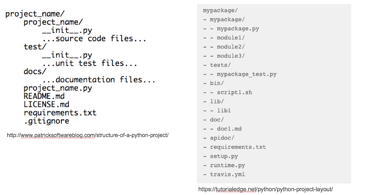Some Common Project Structures ]

• We will have the following project structure.

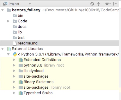Initial Project Structure ]

Simulate a Sequence of At-Bats

• This is just multiple iterations of flipping the coin.

simulator_core.random_set

# Flips the biased coin N-times and returns the
# vector of results
def random_set(probability, count):
    result = []
    
    for i in range(0,count):
        event = biased_coin(probability)
        result.append(event)
        
    return result

/tests/unit_test_sequence

• We will run a simple "eyeball test" to see if the sequences look reasonable.

• We will also test the average behavior.

def eyeball_event_str():
    event_stream = random_set(0.333,20)
    print("Event stream = ", event_stream)
    
def test_event_string_avg():
    event_stream = random_set(0.333, 10000)
    count = len(event_stream)
    total = 0
    for i in range(0, count):
        total = total + event_stream[i]

    avg = total / count
    print("test_event_string: avg = ", avg, " element count = ", count)

    
eyeball_event_str()
test_event_string_avg()

Event stream =  [1, 0, 0, 0, 1, 1, 1, 1, 0, 1, 1, 0, 0, 1, 1, 0, 1, 0, 0, 1]
test_event_string: avg =  0.3252  element count =  10000

Compute Slumps

• Simulate a season of at-bats with _randomset()

• Process the season and find the hitless streaks.

simulator_core.failure_streak_lengths

• My typing and debugging the code while you watch is tedious.

• Instead I will step through and comment the code to explain the logic.

def failure_streak_lengths(event_stream):
    result = []
    on_a_streak = False;
    count = len(event_stream)

    on_a_streak = False
    current_fail_streak = 0

    for i in range(0,count):
        current_event = event_stream[i]

        if current_event == 0:
            if on_a_streak == False:
                on_a_streak = True
                current_fail_streak = 1
            else:
                current_fail_streak = current_fail_streak + 1
        else:
            if on_a_streak == True:
                on_a_streak = False;
                result.append(current_fail_streak)
                current_fail_streak = 0
    else:
        if on_a_streak == True:
            result.append(current_fail_streak)
                
    return result

/tests/unit_test_length

def eyeball_streak_length():
    event_stream = random_set(0.333, 30)
    print("Event stream = ", event_stream)
    fail_streaks = failure_streak_lengths(event_stream)
    print("Hitless streaks = ", fail_streaks)

eyeball_streak_length()

Event stream =  [0, 1, 0, 0, 0, 0, 0, 1, 0, 1, 0, 0, 1, 0, 0, 1, 0, 0, 1, 0, 0, 0, 0, 0, 0, 0, 1, 0, 0, 0]
Hitless streaks =  [1, 5, 1, 2, 2, 2, 7, 3]

Slumps per Season

• Well, I can find the individual hitless streaks.

• What I want is the distribution or histogram of the hitless streak lengths/season.

• There is nothing special about "baseball hitless streaks," and I will just continue to use my various biased coin functions.

simulator_core.histogram_streak_lengths

def histogram_streak_lengths(lengths):
    result = []
    max_fails = max(lengths)

    for j in range(0,max_fails+1):
        result.append(0)

    for i in range(0,len(lengths)):
        fails = lengths[i]
        result[fails] = result[fails] + 1
        
    return result

/tests/test_histogram

def eyeball_histogram():
    event_stream = random_set(0.250, 30)
    print("Event stream = ", event_stream)
    fail_streaks = failure_streak_lengths(event_stream)
    print("Streaks = ", fail_streaks)
    fail_histo = histogram_streak_lengths(fail_streaks)
    print("Histogram = ", fail_histo)

eyeball_histogram()

Event stream =  [0, 1, 0, 0, 0, 0, 0, 0, 0, 0, 1, 0, 0, 0, 0, 0, 1, 0, 0, 1, 0, 0, 0, 0, 0, 0, 0, 0, 0, 0]
Streaks =  [1, 8, 5, 2, 10]
Histogram =  [0, 1, 1, 0, 0, 1, 0, 0, 1, 0, 1]

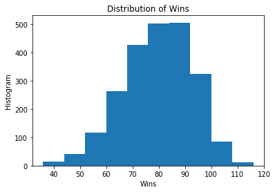
Status Check

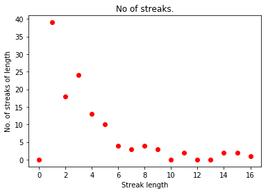
• I can now simulate a season and report on number of streaks of a given length.

• There are about 600 at-bats in a season.

def simulate_season(avg, no_at_bats):
    event_stream = random_set(avg, no_at_bats)
    fail_streaks = failure_streak_lengths(event_stream)
    fail_histo = histogram_streak_lengths(fail_streaks)
    return fail_histo

ab = 600
avg = 0.250
print("Simulating seasons with ", ab, "at bats and batting average ", avg)
histo = simulate_season(avg, ab)

for i in range(0,len(histo)):
    print("Streak length ", i, " no of occurences ", histo[i])
    

Simulating seasons with  600 at bats and batting average  0.25
Streak length  0  no of occurences  0
Streak length  1  no of occurences  39
Streak length  2  no of occurences  18
Streak length  3  no of occurences  24
Streak length  4  no of occurences  13
Streak length  5  no of occurences  10
Streak length  6  no of occurences  4
Streak length  7  no of occurences  3
Streak length  8  no of occurences  4
Streak length  9  no of occurences  3
Streak length  10  no of occurences  0
Streak length  11  no of occurences  2
Streak length  12  no of occurences  0
Streak length  13  no of occurences  0
Streak length  14  no of occurences  2
Streak length  15  no of occurences  2
Streak length  16  no of occurences  1

import matplotlib.pyplot as plt

def add_to_plot(x,y):
    result = False
    if (isinstance(x,int) or isinstance(x,float)) and \
        (isinstance(y,int) or isinstance(y,float)):
        plt.plot(x,y,"ro")
        result = True
        
    return result

for i in range(0,len(histo)):
    add_to_plot(i,histo[i])
   
plt.title("No of streaks.")
plt.xlabel("Streak length")
plt.ylabel("No. of streaks of length")
plt.show()

Next Steps

• Simulate many seasons.

• Aggregating each season allows me to compute the expected number of hitless streaks of length n per season.

• Then can determine if slumps really occur, or are just part of statistical behavior.